Fast Spectral Correlation (FSC) Interferometry
Multiple Beam Interferometry and Traditional Spectral Evaluation
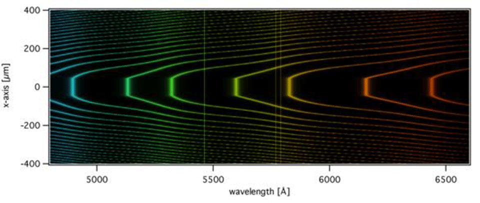
The two cylindrically curved mica surfaces in the Surface Forces Apparatus (SFA) are back-silvered, forming an optical interferometer. The gap or confined film between the two mica surfaces naturally forms an optical layer in the middle of the interferometer. A change of the optical path within this middle layer modifies the conditions for constructive interference and fringes of equal chromatic order (FECO) will be shifted in wavelength. Spectral evaluation is required to determine the wavelegth(s) of one or multiple FECOs. Measurement of FECO wavelength(s) is often done manually by adjusting a grating onto the FECO in an eyepiece that can be moved sidewise with a micrometer. Using optics theory, this wavelength(s) information can be used to calculate the optical parameters of the gap layer - these are the layer thickness, D and the layer refractive index, n. The technique of measuring distance and refractive index in or between thin films is commonly called multiple beam interferometry (MBI) and is intrinsic to all interferometric SFAs.
The traditional spectral evaluation involves manual measurement of the wavelength, l, of one FECO and a linearized approximation to calculate D(l) and/or n(l). If the manually tracked fringe has an odd chromatic order, its wavelength shifts only when D is varied. Even-ordered fringes, however, shift in wavelength for both variations in D and n. Therefore, only every other interference fringe is sensitive to variations of refractive index, which allows one to extract both parameters at the same time. Nevertheless, measurement of refractive index is not commonly practiced and only a few systematic measurements of refractive index have been published in the literature. Due to increasing measurement errors for thinner films, manual FECO-wavelength(s) determination effectively limits determination of the refractive index to films thicker than some 25-50nm.
Automated FECO Detection
The extended Surface Forces Apparatus uses a high-resolution CCD camera to acquire the interference spectrum of the light from the interferometer. Such a spectrum is measured with 5000 pixels (7µm x 7µm) over the entire focal plane of the analyzing spectrograph (Figure 2). The pixel data is automatically transfered to the computer, which determines the exact wavelength of all FECO within the available spectral range. The calibration of pixel position versus wavelength is done using a high-aperture mercury calibration lamp prior to the actual measurement. A non-linear calibration is used to account for the trigonometric nature of the dispersion in the spectrograph. Typical calibration errors are in the order of 3-8pm (wavelength).
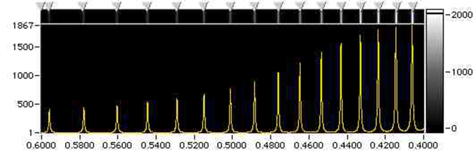
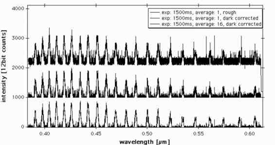
FECO peak determination is realized with a specially developed peak detection algorithm. Parameters that need to be adjusted are approximate peak width and detection level. To reduce statistical errors in FECO peak detection, different digital signal filter steps are available as illustrated in Figure 3.
With a 450-Watt Xenon arc lamp and 1000ms exposure, one can readily obtain a FECO peak determination with a standard deviation in the order of 0.05 pixel (Dl=2pm). This high precision is only possible when the shape of the peaks is accounted for. The typical range of FECO peak widths is 15-50 pixels in our system.
Principle of Fast Spectral Correlation (FSC) Interferometry
Once the FECO peak positions, li, are determined, the software performs a numerical conversion to extract film thickness, D, and refractive index, n, of any desired layer in the interferometer. This procedure requires however that all other optical layers in the interferometer be fully characterized. It is for this reason that FSC-evaluation requires the measurement of the optical zero (i.e. mica thickness), before a film is introduced between the mica sheets. The numerical conversion is directly based on the multilayer matrix method (MMM), which is commonly used to calculate the transmissivity of multilayer interferometric filters. In contrast to the widely used linearized analytical approximation, the MMM has a number of key advantages. However, the MMM can only be used to calculate the transmission spectrum, I(l), if all parameters describing the optical multilayer interferometer are already known. Unfortunately, an analytical inversion of the multilayer matrix method is not available:
ADVANTAGES of the Multilayer Matrix Method
- the calculation is exact (no approximations)
- there are no limitations as to the maximal film thickness
- any number of optical layers in the interferometer can be considered
- calculations can be performed for both symmetric and asymmetric interferometers
- optical layers with complex refractive index can be included (absorbing or emitting layers)
- issues of dispersion and phase change are automatically accounted for (e.g. variable silver mirror thickness)
DISADVANTAGES of the Multilayer Matrix Method
- the MMM has no analytical inversion
To use the MMM efficiently for automated spectral evaluation, it is thus necessary to implement a numerical inversion. If all but a few (e.g. 1 or 2) parameters of an interferometer are known, the MMM can be used to find the best fit between theory and a measured spectrum. Such a fitting algorithm can be based on maximizing the match between measured and calculated spectra. Maximizing the correlation function between the two spectra would be the most straightforward method. The only limitation would be speed of calculation, because the spectral correlation must be calculated many times during a fitting procedure. Fast Spectral Correlation (FSC) can reduce this computational effort by about two or three orders of magnitude while preserving all important spectral information. The principle of FSC is illustrated in Figure 4.

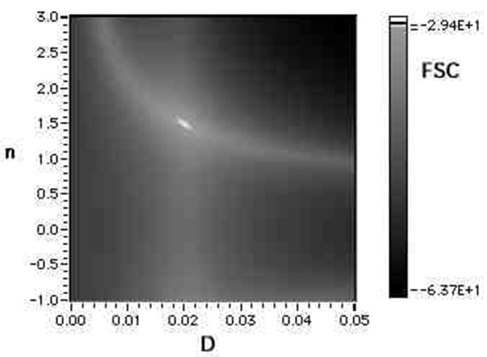
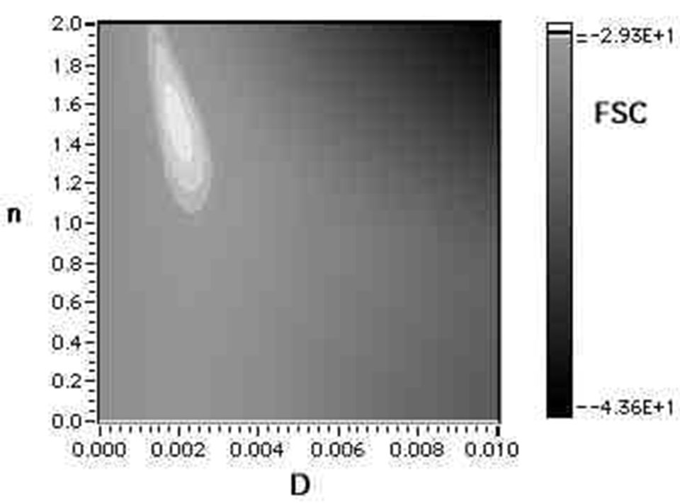
As we have now all necesary tools at hand to implement a fast and efficient inversion of the MMM, it is still important to know more about the FSC in terms of fitting a given set of parameters. Almost any combination of parameters can be fitted with the limitation that the result may become less reliable with an increasing number of unknown parameters. The examples shown in figures 5a-c illustrate how one can use FSC to simultaneously extract film thickness and refractive index of the medium between two sheets of mica. This is one of the most commonly encountered situations.

Precision of Fast Spectral Correlation
Figures 5 illustrate a typical topology of the FSC in the (D, n) plane, where D is the thickness of the gap layer and n its refractive index. The next step is to implement a fitting algorithm that uses FSC to find the desired solution. Generally it is possible to design a fitting algorithm that searches for any combination of unknown parameters in the matrix that describes the interferometer. Such a general fitting algorithm is difficult to implement since the topology of FSC may be very complex in certain variables. Two situations are however of special importance in the context of eSFA measurements.
The D-evaluation
In the first situation, all parameters of the multilayer matrix are known, except for the thickness of the gap medium (i.e. surface separation). Here, the task is to evaluate the interference spectrum in terms of D at a constant n. In Figures 5, this corresponds to searching the point of maximal FSC along a horizontal line (i.e. n=constant). The statistical errors of this method mainly arise from an imperfect determination of interference fringe peak wavelengths. Figure 6 illustrates the standard deviation of the D-evaluation under the assumption that each fringe wavelength is determined with a standard deviation of 10pm (gaussian noise). This is a rather pessimistic assumption since the FECO detection has a typical standard deviation of 1-3pm.
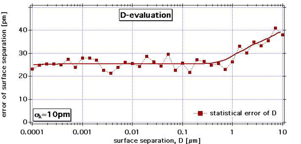
The standard deviation of distance measurement (D-evaluation) is in the order of 25pm over a wide distance range. This is possible because for larger distances we can detect more fringes in the available spectral range. If M is the number of detected fringes, then the statistical error can be reduced by a factor of M^0.5. For distances above D=1µm, we observe a roughly logarithmically increase. Up to a distance of D=10µm the standard deviation remains below 40pm.
The Dn-Evaluation
The second common situation involves simultaneous determination of D and n (Dn-evaluation). This corresponds to finding the absolute maximum of the FSC in the (D, n)-plane. The statistical errors of both matrix variables, D and n, is illustrated in figure 7. The calculation is based on the assumption that the fringe detection is made with a standard deviation of 10pm (gaussian noise).
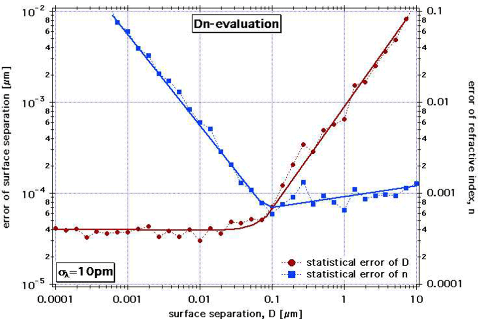
Figure 7 clearly shows that there is a trade-off between precision of D and precision of n. Namely determination of D is more precise for small surface separations - a key factor for the SFA technique in general. The statistical error of n is however smallest for surface separations around 100nm. The useful range of the Dn-evaluation is thus effectively limited to a range from 1nm to 100nm. For surface separation exceeding 100nm it is therefore always better to use the D-evaluation to determine D.
Errors Due to Mechanical Vibrations
Since one surface is mounted on a compliant spring in the SFA, one can readily observe mechanical vibrations that affect the surface separation. We are using an air-cushioned anti-vibration table. Nevertheless, mechanical vibrations are noticeable in configurations involving a weak spring and in a low-viscous medium such as air. In this worst case we observe a mechanical vibration of the surfaces with amplitude of several nm and in the frequency range 30-100Hz (i.e. resonance given by spring constant and sample mass). Assuming that the oscillation is, on average, symmetric around the true equilibrium surface separation, it is possible to average it out using effective CCD exposure times between 1000ms and 3000ms and multi-exposure averaging. The assumption of symmetric oscillations can be inaccurate in attractive surface potentials and for weak repulsive surface forces. For measurements in fluids, the vibration is barely noticeable and when the surfaces come into contact (loading cycle) the vibration vanishes.
To test the performance of D-evaluation and Dn-evaluation in a realistic worst-case scenario, we have measured distance, D, (D-evaluation) and refractive index, n, (Dn-evaluation) in air at a surface separation around 300nm. The spring constant was 1002±23N/m and the sample mass is about 2.5 grams, which results in a mechanical resonance at a frequency n~100Hz.

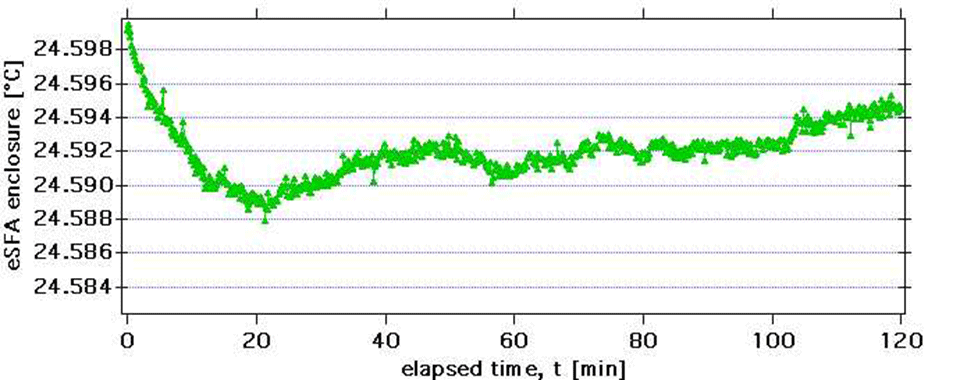
The standard deviation of n is smaller than 0.002 and the standard deviation of D (D-evaluation) is in the order of 70pm. The instrumental drift rate is less than 0.1Å/minute. The small modulations in D are due to small variations in temperature ±0.002°C in the thermal enclosure of the eSFA. The temperature was measured simultaneously and is shown in Figure 9 below.
Scanning eSFA
The measurement of interference spectra with a linear CCD is different from the manual measurement (with grating in eyepiece) inasmuch as the manual measurement yields a mean value for the FECO wavelength in the contact zone, whereas the CCD can provide a measurement at a point (optical point probe). The lateral resolution of this optical probe is about 1µm. With a calibrated motion of CCD and a deflection mirror, it is thus possible to scan the optical probe laterally and hence produce a three-dimensional representation of the entire contact geometry. Figure 10 below illustrates such a scan, which was taken with the optical point probe at over 1000 different lateral locations. With this new technique it is possible to measure the film thickness and refractive index of a confined medium as well as the contact geometry at any point in the vicinity of the contact zone.
![Figure 10: Animated 3D-scan of an elastically deformed mica-mica contact zone under an external load F=0.5mNin the eSFA. All units in [µm].](/research/surface-forces/the-extended-surface-forces-apparatus-esfa/fast-spectral-correlation-fsc-interferometry/_jcr_content/par/fullwidthimage_981378191/image.imageformat.1286.127344901.gif)
(You may have to press "RELOAD" in your browser to restart the animation.)